Observação

Clique aqui para baixar o código de exemplo completo

Personalizando Matplotlib com folhas de estilo e rcParams #

Dicas para personalizar as propriedades e estilos padrão do Matplotlib.

Existem três maneiras de personalizar o Matplotlib:

Configurando rcParams em tempo de execução .

Usando folhas de estilo .

Alterando seu arquivo matplotlibrc .

A definição de rcParams em tempo de execução tem precedência sobre as folhas de estilo, as folhas de estilo têm precedência sobre os matplotlibrcarquivos.

Configurações rc de tempo de execução #

Você pode alterar dinamicamente as configurações padrão de rc (configuração de tempo de execução) em um script python ou interativamente a partir do shell python. Todas as configurações rc são armazenadas em uma variável semelhante a um dicionário chamada matplotlib.rcParams, que é global para o pacote matplotlib. Consulte matplotlib.rcParamspara obter uma lista completa de rcParams configuráveis. rcParams pode ser modificado diretamente, por exemplo:

import numpy as np
import matplotlib.pyplot as plt
import matplotlib as mpl
from cycler import cycler
mpl.rcParams['lines.linewidth'] = 2
mpl.rcParams['lines.linestyle'] = '--'
data = np.random.randn(50)
plt.plot(data)

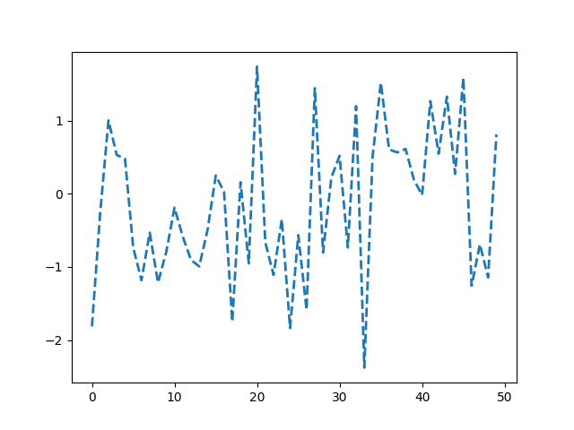
[<matplotlib.lines.Line2D object at 0x7f2cdd6a05b0>]

Observe que, para alterar a plotcor usual, você deve alterar a propriedade prop_cycle dos eixos :

mpl.rcParams['axes.prop_cycle'] = cycler(color=['r', 'g', 'b', 'y'])
plt.plot(data)  # first color is red

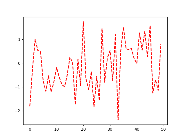
[<matplotlib.lines.Line2D object at 0x7f2cdda41e70>]

O Matplotlib também fornece algumas funções de conveniência para modificar as configurações do rc. matplotlib.rcpode ser usado para modificar várias configurações em um único grupo de uma só vez, usando argumentos de palavra-chave:

mpl.rc('lines', linewidth=4, linestyle='-.')
plt.plot(data)

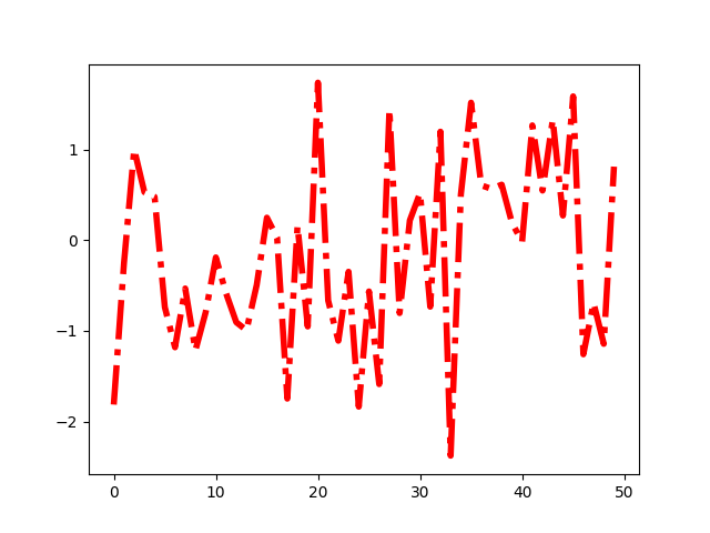
[<matplotlib.lines.Line2D object at 0x7f2cdd6a0b50>]

Configurações rc temporárias #

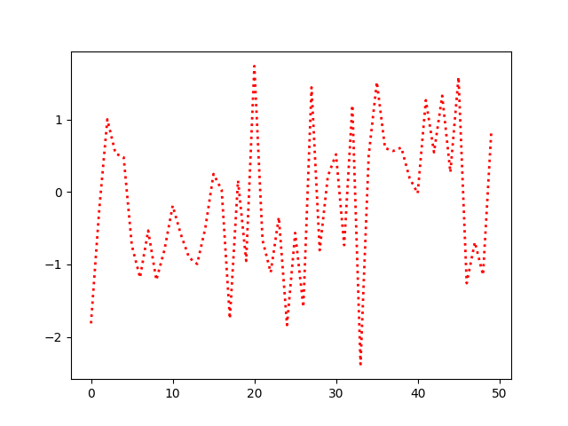
O matplotlib.rcParamsobjeto também pode ser alterado temporariamente usando o matplotlib.rc_contextgerenciador de contexto:

with mpl.rc_context({'lines.linewidth': 2, 'lines.linestyle': ':'}):
    plt.plot(data)

matplotlib.rc_contexttambém pode ser usado como decorador para modificar os padrões dentro de uma função:

@mpl.rc_context({'lines.linewidth': 3, 'lines.linestyle': '-'})
def plotting_function():
    plt.plot(data)

plotting_function()

matplotlib.rcdefaultsrestaurará as configurações padrão do Matplotlib padrão.

Há algum grau de validação ao definir os valores de rcParams, consulte matplotlib.rcsetuppara obter detalhes.

Usando folhas de estilo #

Outra maneira de alterar a aparência visual dos gráficos é definir o rcParams em uma chamada folha de estilo e importar essa folha de estilo com matplotlib.style.use. Dessa forma, você pode alternar facilmente entre diferentes estilos simplesmente alterando a folha de estilo importada. Uma folha de estilo se parece com um arquivo matplotlibrc , mas em uma folha de estilo você só pode definir rcParams relacionados ao estilo real de um gráfico. Outros rcParams, como backend , serão ignorados. matplotlibrcsuportam todos os arquivos rcParams. A lógica por trás disso é tornar as folhas de estilo portáteis entre diferentes máquinas sem ter que se preocupar com dependências que podem ou não estar instaladas em outra máquina. Para obter uma lista completa de rcParams, consulte matplotlib.rcParams. Para obter uma lista de rcParams que são ignorados nas folhas de estilo, consultematplotlib.style.use.

Há vários estilos predefinidos fornecidos pelo Matplotlib . Por exemplo, há um estilo predefinido chamado "ggplot", que emula a estética do ggplot (um pacote de plotagem popular para R ). Para usar este estilo, adicione:

plt.style.use('ggplot')

Para listar todos os estilos disponíveis, use:

print(plt.style.available)

['Solarize_Light2', '_classic_test_patch', '_mpl-gallery', '_mpl-gallery-nogrid', 'bmh', 'classic', 'dark_background', 'fast', 'fivethirtyeight', 'ggplot', 'grayscale', 'seaborn-v0_8', 'seaborn-v0_8-bright', 'seaborn-v0_8-colorblind', 'seaborn-v0_8-dark', 'seaborn-v0_8-dark-palette', 'seaborn-v0_8-darkgrid', 'seaborn-v0_8-deep', 'seaborn-v0_8-muted', 'seaborn-v0_8-notebook', 'seaborn-v0_8-paper', 'seaborn-v0_8-pastel', 'seaborn-v0_8-poster', 'seaborn-v0_8-talk', 'seaborn-v0_8-ticks', 'seaborn-v0_8-white', 'seaborn-v0_8-whitegrid', 'tableau-colorblind10']

Definindo seu próprio estilo #

Você pode criar estilos personalizados e usá-los chamando style.usecom o caminho ou URL para a folha de estilo.

Por exemplo, você pode querer criar ./images/presentation.mplstylecom o seguinte:

axes.titlesize : 24
axes.labelsize : 20
lines.linewidth : 3
lines.markersize : 10
xtick.labelsize : 16
ytick.labelsize : 16

Então, quando você quiser adaptar uma plotagem projetada para um papel para uma que fique bem em uma apresentação, basta adicionar:

>>> import matplotlib.pyplot as plt
>>> plt.style.use('./images/presentation.mplstyle')

Como alternativa, você pode tornar seu estilo conhecido no Matplotlib colocando seu <style-name>.mplstylearquivo em mpl_configdir/stylelib. Você pode carregar sua folha de estilo personalizada com uma chamada para style.use(<style-name>). Por padrão mpl_configdirdeve ser ~/.config/matplotlib, mas você pode verificar onde está o seu com matplotlib.get_configdir(); pode ser necessário criar este diretório. Você também pode alterar o diretório onde o Matplotlib procura a pasta stylelib/ definindo aMPLCONFIGDIRvariável de ambiente, consulte a configuração do matplotlib e os locais do diretório de cache .

Observe que uma folha de estilo personalizada mpl_configdir/stylelibsubstituirá uma folha de estilo definida por Matplotlib se os estilos tiverem o mesmo nome.

Uma vez que seu <style-name>.mplstylearquivo esteja no formato apropriado mpl_configdir, você pode especificar seu estilo com:

>>> import matplotlib.pyplot as plt
>>> plt.style.use(<style-name>)

Estilos de composição #

As folhas de estilo são projetadas para serem compostas juntas. Assim, você pode ter uma folha de estilo que personaliza cores e uma folha de estilo separada que altera o tamanho dos elementos para apresentações. Esses estilos podem ser facilmente combinados passando uma lista de estilos:

>>> import matplotlib.pyplot as plt
>>> plt.style.use(['dark_background', 'presentation'])

Observe que os estilos mais à direita substituirão os valores que já estão definidos pelos estilos à esquerda.

Estilização temporária #

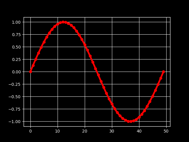
Se você deseja usar apenas um estilo para um bloco de código específico, mas não deseja alterar o estilo global, o pacote de estilo fornece um gerenciador de contexto para limitar suas alterações a um escopo específico. Para isolar suas alterações de estilo, você pode escrever algo como o seguinte:

with plt.style.context('dark_background'):
    plt.plot(np.sin(np.linspace(0, 2 * np.pi)), 'r-o')
plt.show()

o `matplotlibrc`arquivo #

Matplotlib usa matplotlibrcarquivos de configuração para personalizar todos os tipos de propriedades, que chamamos de 'configurações rc' ou 'parâmetros rc'. Você pode controlar os padrões de quase todas as propriedades no Matplotlib: tamanho da figura e DPI, largura da linha, cor e estilo, eixos, propriedades de eixo e grade, propriedades de texto e fonte e assim por diante. O matplotlibrcé lido na inicialização para configurar o Matplotlib. O Matplotlib procura matplotlibrcem quatro locais, na seguinte ordem:

matplotlibrcno diretório de trabalho atual, geralmente usado para personalizações específicas que você não deseja aplicar em outro lugar.
$MATPLOTLIBRCse for um arquivo, senão $MATPLOTLIBRC/matplotlibrc.
Em seguida, ele procura em um local específico do usuário, dependendo da sua plataforma:
- No Linux e FreeBSD, ele verifica .config/matplotlib/matplotlibrc(ou $XDG_CONFIG_HOME/matplotlib/matplotlibrc) se você personalizou seu ambiente.
- Em outras plataformas, ele aparece em .matplotlib/matplotlibrc.
Consulte a configuração do matplotlib e os locais do diretório de cache .
INSTALL/matplotlib/mpl-data/matplotlibrc, onde INSTALLé algo como /usr/lib/python3.9/site-packagesno Linux e talvez C:\Python39\Lib\site-packagesno Windows. Toda vez que você instalar o matplotlib, este arquivo será substituído, portanto, se você deseja que suas personalizações sejam salvas, mova este arquivo para o diretório matplotlib específico do usuário.

Depois que um matplotlibrcarquivo for encontrado, ele não pesquisará nenhum dos outros caminhos. Quando uma folha de estilo é fornecida com style.use('<path>/<style-name>.mplstyle'), as configurações especificadas na folha de estilo têm precedência sobre as configurações no matplotlibrcarquivo.

Para exibir de onde o arquivo atualmente ativo matplotlibrcfoi carregado, pode-se fazer o seguinte:

>>> import matplotlib
>>> matplotlib.matplotlib_fname()
'/home/foo/.config/matplotlib/matplotlibrc'

Veja abaixo um exemplo de arquivo matplotlibrc e veja matplotlib.rcParamsuma lista completa de rcParams configuráveis.

`matplotlibrc`O arquivo padrão #

#### MATPLOTLIBRC FORMAT

## NOTE FOR END USERS: DO NOT EDIT THIS FILE!
##
## This is a sample Matplotlib configuration file - you can find a copy
## of it on your system in site-packages/matplotlib/mpl-data/matplotlibrc
## (relative to your Python installation location).
## DO NOT EDIT IT!
##
## If you wish to change your default style, copy this file to one of the
## following locations:
##     Unix/Linux:
##         $HOME/.config/matplotlib/matplotlibrc OR
##         $XDG_CONFIG_HOME/matplotlib/matplotlibrc (if $XDG_CONFIG_HOME is set)
##     Other platforms:
##         $HOME/.matplotlib/matplotlibrc
## and edit that copy.
##
## See https://matplotlib.org/stable/tutorials/introductory/customizing.html#customizing-with-matplotlibrc-files
## for more details on the paths which are checked for the configuration file.
##
## Blank lines, or lines starting with a comment symbol, are ignored, as are
## trailing comments.  Other lines must have the format:
##     key: val  # optional comment
##
## Formatting: Use PEP8-like style (as enforced in the rest of the codebase).
## All lines start with an additional '#', so that removing all leading '#'s
## yields a valid style file.
##
## Colors: for the color values below, you can either use
##     - a Matplotlib color string, such as r, k, or b
##     - an RGB tuple, such as (1.0, 0.5, 0.0)
##     - a double-quoted hex string, such as "#ff00ff".
##       The unquoted string ff00ff is also supported for backward
##       compatibility, but is discouraged.
##     - a scalar grayscale intensity such as 0.75
##     - a legal html color name, e.g., red, blue, darkslategray
##
## String values may optionally be enclosed in double quotes, which allows
## using the comment character # in the string.
##
## This file (and other style files) must be encoded as utf-8.
##
## Matplotlib configuration are currently divided into following parts:
##     - BACKENDS
##     - LINES
##     - PATCHES
##     - HATCHES
##     - BOXPLOT
##     - FONT
##     - TEXT
##     - LaTeX
##     - AXES
##     - DATES
##     - TICKS
##     - GRIDS
##     - LEGEND
##     - FIGURE
##     - IMAGES
##     - CONTOUR PLOTS
##     - ERRORBAR PLOTS
##     - HISTOGRAM PLOTS
##     - SCATTER PLOTS
##     - AGG RENDERING
##     - PATHS
##     - SAVING FIGURES
##     - INTERACTIVE KEYMAPS
##     - ANIMATION

##### CONFIGURATION BEGINS HERE


## ***************************************************************************
## * BACKENDS                                                                *
## ***************************************************************************
## The default backend.  If you omit this parameter, the first working
## backend from the following list is used:
##     MacOSX QtAgg Gtk4Agg Gtk3Agg TkAgg WxAgg Agg
## Other choices include:
##     QtCairo GTK4Cairo GTK3Cairo TkCairo WxCairo Cairo
##     Qt5Agg Qt5Cairo Wx  # deprecated.
##     PS PDF SVG Template
## You can also deploy your own backend outside of Matplotlib by referring to
## the module name (which must be in the PYTHONPATH) as 'module://my_backend'.
##backend: Agg

## The port to use for the web server in the WebAgg backend.
#webagg.port: 8988

## The address on which the WebAgg web server should be reachable
#webagg.address: 127.0.0.1

## If webagg.port is unavailable, a number of other random ports will
## be tried until one that is available is found.
#webagg.port_retries: 50

## When True, open the web browser to the plot that is shown
#webagg.open_in_browser: True

## If you are running pyplot inside a GUI and your backend choice
## conflicts, we will automatically try to find a compatible one for
## you if backend_fallback is True
#backend_fallback: True

#interactive: False
#toolbar:     toolbar2  # {None, toolbar2, toolmanager}
#timezone:    UTC       # a pytz timezone string, e.g., US/Central or Europe/Paris


## ***************************************************************************
## * LINES                                                                   *
## ***************************************************************************
## See https://matplotlib.org/api/artist_api.html#module-matplotlib.lines
## for more information on line properties.
#lines.linewidth: 1.5               # line width in points
#lines.linestyle: -                 # solid line
#lines.color:     C0                # has no affect on plot(); see axes.prop_cycle
#lines.marker:          None        # the default marker
#lines.markerfacecolor: auto        # the default marker face color
#lines.markeredgecolor: auto        # the default marker edge color
#lines.markeredgewidth: 1.0         # the line width around the marker symbol
#lines.markersize:      6           # marker size, in points
#lines.dash_joinstyle:  round       # {miter, round, bevel}
#lines.dash_capstyle:   butt        # {butt, round, projecting}
#lines.solid_joinstyle: round       # {miter, round, bevel}
#lines.solid_capstyle:  projecting  # {butt, round, projecting}
#lines.antialiased: True            # render lines in antialiased (no jaggies)

## The three standard dash patterns.  These are scaled by the linewidth.
#lines.dashed_pattern: 3.7, 1.6
#lines.dashdot_pattern: 6.4, 1.6, 1, 1.6
#lines.dotted_pattern: 1, 1.65
#lines.scale_dashes: True

#markers.fillstyle: full  # {full, left, right, bottom, top, none}

#pcolor.shading: auto
#pcolormesh.snap: True  # Whether to snap the mesh to pixel boundaries. This is
                        # provided solely to allow old test images to remain
                        # unchanged. Set to False to obtain the previous behavior.

## ***************************************************************************
## * PATCHES                                                                 *
## ***************************************************************************
## Patches are graphical objects that fill 2D space, like polygons or circles.
## See https://matplotlib.org/api/artist_api.html#module-matplotlib.patches
## for more information on patch properties.
#patch.linewidth:       1.0    # edge width in points.
#patch.facecolor:       C0
#patch.edgecolor:       black  # if forced, or patch is not filled
#patch.force_edgecolor: False  # True to always use edgecolor
#patch.antialiased:     True   # render patches in antialiased (no jaggies)


## ***************************************************************************
## * HATCHES                                                                 *
## ***************************************************************************
#hatch.color:     black
#hatch.linewidth: 1.0


## ***************************************************************************
## * BOXPLOT                                                                 *
## ***************************************************************************
#boxplot.notch:       False
#boxplot.vertical:    True
#boxplot.whiskers:    1.5
#boxplot.bootstrap:   None
#boxplot.patchartist: False
#boxplot.showmeans:   False
#boxplot.showcaps:    True
#boxplot.showbox:     True
#boxplot.showfliers:  True
#boxplot.meanline:    False

#boxplot.flierprops.color:           black
#boxplot.flierprops.marker:          o
#boxplot.flierprops.markerfacecolor: none
#boxplot.flierprops.markeredgecolor: black
#boxplot.flierprops.markeredgewidth: 1.0
#boxplot.flierprops.markersize:      6
#boxplot.flierprops.linestyle:       none
#boxplot.flierprops.linewidth:       1.0

#boxplot.boxprops.color:     black
#boxplot.boxprops.linewidth: 1.0
#boxplot.boxprops.linestyle: -

#boxplot.whiskerprops.color:     black
#boxplot.whiskerprops.linewidth: 1.0
#boxplot.whiskerprops.linestyle: -

#boxplot.capprops.color:     black
#boxplot.capprops.linewidth: 1.0
#boxplot.capprops.linestyle: -

#boxplot.medianprops.color:     C1
#boxplot.medianprops.linewidth: 1.0
#boxplot.medianprops.linestyle: -

#boxplot.meanprops.color:           C2
#boxplot.meanprops.marker:          ^
#boxplot.meanprops.markerfacecolor: C2
#boxplot.meanprops.markeredgecolor: C2
#boxplot.meanprops.markersize:       6
#boxplot.meanprops.linestyle:       --
#boxplot.meanprops.linewidth:       1.0


## ***************************************************************************
## * FONT                                                                    *
## ***************************************************************************
## The font properties used by `text.Text`.
## See https://matplotlib.org/api/font_manager_api.html for more information
## on font properties.  The 6 font properties used for font matching are
## given below with their default values.
##
## The font.family property can take either a single or multiple entries of any
## combination of concrete font names (not supported when rendering text with
## usetex) or the following five generic values:
##     - 'serif' (e.g., Times),
##     - 'sans-serif' (e.g., Helvetica),
##     - 'cursive' (e.g., Zapf-Chancery),
##     - 'fantasy' (e.g., Western), and
##     - 'monospace' (e.g., Courier).
## Each of these values has a corresponding default list of font names
## (font.serif, etc.); the first available font in the list is used.  Note that
## for font.serif, font.sans-serif, and font.monospace, the first element of
## the list (a DejaVu font) will always be used because DejaVu is shipped with
## Matplotlib and is thus guaranteed to be available; the other entries are
## left as examples of other possible values.
##
## The font.style property has three values: normal (or roman), italic
## or oblique.  The oblique style will be used for italic, if it is not
## present.
##
## The font.variant property has two values: normal or small-caps.  For
## TrueType fonts, which are scalable fonts, small-caps is equivalent
## to using a font size of 'smaller', or about 83%% of the current font
## size.
##
## The font.weight property has effectively 13 values: normal, bold,
## bolder, lighter, 100, 200, 300, ..., 900.  Normal is the same as
## 400, and bold is 700.  bolder and lighter are relative values with
## respect to the current weight.
##
## The font.stretch property has 11 values: ultra-condensed,
## extra-condensed, condensed, semi-condensed, normal, semi-expanded,
## expanded, extra-expanded, ultra-expanded, wider, and narrower.  This
## property is not currently implemented.
##
## The font.size property is the default font size for text, given in points.
## 10 pt is the standard value.
##
## Note that font.size controls default text sizes.  To configure
## special text sizes tick labels, axes, labels, title, etc., see the rc
## settings for axes and ticks.  Special text sizes can be defined
## relative to font.size, using the following values: xx-small, x-small,
## small, medium, large, x-large, xx-large, larger, or smaller

#font.family:  sans-serif
#font.style:   normal
#font.variant: normal
#font.weight:  normal
#font.stretch: normal
#font.size:    10.0

#font.serif:      DejaVu Serif, Bitstream Vera Serif, Computer Modern Roman, New Century Schoolbook, Century Schoolbook L, Utopia, ITC Bookman, Bookman, Nimbus Roman No9 L, Times New Roman, Times, Palatino, Charter, serif
#font.sans-serif: DejaVu Sans, Bitstream Vera Sans, Computer Modern Sans Serif, Lucida Grande, Verdana, Geneva, Lucid, Arial, Helvetica, Avant Garde, sans-serif
#font.cursive:    Apple Chancery, Textile, Zapf Chancery, Sand, Script MT, Felipa, Comic Neue, Comic Sans MS, cursive
#font.fantasy:    Chicago, Charcoal, Impact, Western, Humor Sans, xkcd, fantasy
#font.monospace:  DejaVu Sans Mono, Bitstream Vera Sans Mono, Computer Modern Typewriter, Andale Mono, Nimbus Mono L, Courier New, Courier, Fixed, Terminal, monospace


## ***************************************************************************
## * TEXT                                                                    *
## ***************************************************************************
## The text properties used by `text.Text`.
## See https://matplotlib.org/api/artist_api.html#module-matplotlib.text
## for more information on text properties
#text.color: black

## FreeType hinting flag ("foo" corresponds to FT_LOAD_FOO); may be one of the
## following (Proprietary Matplotlib-specific synonyms are given in parentheses,
## but their use is discouraged):
## - default: Use the font's native hinter if possible, else FreeType's auto-hinter.
##            ("either" is a synonym).
## - no_autohint: Use the font's native hinter if possible, else don't hint.
##                ("native" is a synonym.)
## - force_autohint: Use FreeType's auto-hinter.  ("auto" is a synonym.)
## - no_hinting: Disable hinting.  ("none" is a synonym.)
#text.hinting: force_autohint

#text.hinting_factor: 8  # Specifies the amount of softness for hinting in the
                         # horizontal direction.  A value of 1 will hint to full
                         # pixels.  A value of 2 will hint to half pixels etc.
#text.kerning_factor: 0  # Specifies the scaling factor for kerning values.  This
                         # is provided solely to allow old test images to remain
                         # unchanged.  Set to 6 to obtain previous behavior.
                         # Values  other than 0 or 6 have no defined meaning.
#text.antialiased: True  # If True (default), the text will be antialiased.
                         # This only affects raster outputs.
#text.parse_math: True  # Use mathtext if there is an even number of unescaped
                        # dollar signs.


## ***************************************************************************
## * LaTeX                                                                   *
## ***************************************************************************
## For more information on LaTeX properties, see
## https://matplotlib.org/tutorials/text/usetex.html
#text.usetex: False  # use latex for all text handling. The following fonts
                     # are supported through the usual rc parameter settings:
                     # new century schoolbook, bookman, times, palatino,
                     # zapf chancery, charter, serif, sans-serif, helvetica,
                     # avant garde, courier, monospace, computer modern roman,
                     # computer modern sans serif, computer modern typewriter
#text.latex.preamble:   # IMPROPER USE OF THIS FEATURE WILL LEAD TO LATEX FAILURES
                        # AND IS THEREFORE UNSUPPORTED. PLEASE DO NOT ASK FOR HELP
                        # IF THIS FEATURE DOES NOT DO WHAT YOU EXPECT IT TO.
                        # text.latex.preamble is a single line of LaTeX code that
                        # will be passed on to the LaTeX system. It may contain
                        # any code that is valid for the LaTeX "preamble", i.e.
                        # between the "\documentclass" and "\begin{document}"
                        # statements.
                        # Note that it has to be put on a single line, which may
                        # become quite long.
                        # The following packages are always loaded with usetex,
                        # so beware of package collisions:
                        #   geometry, inputenc, type1cm.
                        # PostScript (PSNFSS) font packages may also be
                        # loaded, depending on your font settings.

## The following settings allow you to select the fonts in math mode.
#mathtext.fontset: dejavusans  # Should be 'dejavusans' (default),
                               # 'dejavuserif', 'cm' (Computer Modern), 'stix',
                               # 'stixsans' or 'custom' (unsupported, may go
                               # away in the future)
## "mathtext.fontset: custom" is defined by the mathtext.bf, .cal, .it, ...
## settings which map a TeX font name to a fontconfig font pattern.  (These
## settings are not used for other font sets.)
#mathtext.bf:  sans:bold
#mathtext.cal: cursive
#mathtext.it:  sans:italic
#mathtext.rm:  sans
#mathtext.sf:  sans
#mathtext.tt:  monospace
#mathtext.fallback: cm  # Select fallback font from ['cm' (Computer Modern), 'stix'
                        # 'stixsans'] when a symbol can not be found in one of the
                        # custom math fonts. Select 'None' to not perform fallback
                        # and replace the missing character by a dummy symbol.
#mathtext.default: it  # The default font to use for math.
                       # Can be any of the LaTeX font names, including
                       # the special name "regular" for the same font
                       # used in regular text.


## ***************************************************************************
## * AXES                                                                    *
## ***************************************************************************
## Following are default face and edge colors, default tick sizes,
## default font sizes for tick labels, and so on.  See
## https://matplotlib.org/api/axes_api.html#module-matplotlib.axes
#axes.facecolor:     white   # axes background color
#axes.edgecolor:     black   # axes edge color
#axes.linewidth:     0.8     # edge line width
#axes.grid:          False   # display grid or not
#axes.grid.axis:     both    # which axis the grid should apply to
#axes.grid.which:    major   # grid lines at {major, minor, both} ticks
#axes.titlelocation: center  # alignment of the title: {left, right, center}
#axes.titlesize:     large   # font size of the axes title
#axes.titleweight:   normal  # font weight of title
#axes.titlecolor:    auto    # color of the axes title, auto falls back to
                             # text.color as default value
#axes.titley:        None    # position title (axes relative units).  None implies auto
#axes.titlepad:      6.0     # pad between axes and title in points
#axes.labelsize:     medium  # font size of the x and y labels
#axes.labelpad:      4.0     # space between label and axis
#axes.labelweight:   normal  # weight of the x and y labels
#axes.labelcolor:    black
#axes.axisbelow:     line    # draw axis gridlines and ticks:
                             #     - below patches (True)
                             #     - above patches but below lines ('line')
                             #     - above all (False)

#axes.formatter.limits: -5, 6  # use scientific notation if log10
                               # of the axis range is smaller than the
                               # first or larger than the second
#axes.formatter.use_locale: False  # When True, format tick labels
                                   # according to the user's locale.
                                   # For example, use ',' as a decimal
                                   # separator in the fr_FR locale.
#axes.formatter.use_mathtext: False  # When True, use mathtext for scientific
                                     # notation.
#axes.formatter.min_exponent: 0  # minimum exponent to format in scientific notation
#axes.formatter.useoffset: True  # If True, the tick label formatter
                                 # will default to labeling ticks relative
                                 # to an offset when the data range is
                                 # small compared to the minimum absolute
                                 # value of the data.
#axes.formatter.offset_threshold: 4  # When useoffset is True, the offset
                                     # will be used when it can remove
                                     # at least this number of significant
                                     # digits from tick labels.

#axes.spines.left:   True  # display axis spines
#axes.spines.bottom: True
#axes.spines.top:    True
#axes.spines.right:  True

#axes.unicode_minus: True  # use Unicode for the minus symbol rather than hyphen.  See
                           # https://en.wikipedia.org/wiki/Plus_and_minus_signs#Character_codes
#axes.prop_cycle: cycler('color', ['1f77b4', 'ff7f0e', '2ca02c', 'd62728', '9467bd', '8c564b', 'e377c2', '7f7f7f', 'bcbd22', '17becf'])
                  # color cycle for plot lines as list of string color specs:
                  # single letter, long name, or web-style hex
                  # As opposed to all other parameters in this file, the color
                  # values must be enclosed in quotes for this parameter,
                  # e.g. '1f77b4', instead of 1f77b4.
                  # See also https://matplotlib.org/tutorials/intermediate/color_cycle.html
                  # for more details on prop_cycle usage.
#axes.xmargin:   .05  # x margin.  See `axes.Axes.margins`
#axes.ymargin:   .05  # y margin.  See `axes.Axes.margins`
#axes.zmargin:   .05  # z margin.  See `axes.Axes.margins`
#axes.autolimit_mode: data  # If "data", use axes.xmargin and axes.ymargin as is.
                            # If "round_numbers", after application of margins, axis
                            # limits are further expanded to the nearest "round" number.
#polaraxes.grid: True  # display grid on polar axes
#axes3d.grid:    True  # display grid on 3D axes


## ***************************************************************************
## * AXIS                                                                    *
## ***************************************************************************
#xaxis.labellocation: center  # alignment of the xaxis label: {left, right, center}
#yaxis.labellocation: center  # alignment of the yaxis label: {bottom, top, center}


## ***************************************************************************
## * DATES                                                                   *
## ***************************************************************************
## These control the default format strings used in AutoDateFormatter.
## Any valid format datetime format string can be used (see the python
## `datetime` for details).  For example, by using:
##     - '%%x' will use the locale date representation
##     - '%%X' will use the locale time representation
##     - '%%c' will use the full locale datetime representation
## These values map to the scales:
##     {'year': 365, 'month': 30, 'day': 1, 'hour': 1/24, 'minute': 1 / (24 * 60)}

#date.autoformatter.year:        %Y
#date.autoformatter.month:       %Y-%m
#date.autoformatter.day:         %Y-%m-%d
#date.autoformatter.hour:        %m-%d %H
#date.autoformatter.minute:      %d %H:%M
#date.autoformatter.second:      %H:%M:%S
#date.autoformatter.microsecond: %M:%S.%f
## The reference date for Matplotlib's internal date representation
## See https://matplotlib.org/examples/ticks_and_spines/date_precision_and_epochs.py
#date.epoch: 1970-01-01T00:00:00
## 'auto', 'concise':
#date.converter:                  auto
## For auto converter whether to use interval_multiples:
#date.interval_multiples:         True

## ***************************************************************************
## * TICKS                                                                   *
## ***************************************************************************
## See https://matplotlib.org/api/axis_api.html#matplotlib.axis.Tick
#xtick.top:           False   # draw ticks on the top side
#xtick.bottom:        True    # draw ticks on the bottom side
#xtick.labeltop:      False   # draw label on the top
#xtick.labelbottom:   True    # draw label on the bottom
#xtick.major.size:    3.5     # major tick size in points
#xtick.minor.size:    2       # minor tick size in points
#xtick.major.width:   0.8     # major tick width in points
#xtick.minor.width:   0.6     # minor tick width in points
#xtick.major.pad:     3.5     # distance to major tick label in points
#xtick.minor.pad:     3.4     # distance to the minor tick label in points
#xtick.color:         black   # color of the ticks
#xtick.labelcolor:    inherit # color of the tick labels or inherit from xtick.color
#xtick.labelsize:     medium  # font size of the tick labels
#xtick.direction:     out     # direction: {in, out, inout}
#xtick.minor.visible: False   # visibility of minor ticks on x-axis
#xtick.major.top:     True    # draw x axis top major ticks
#xtick.major.bottom:  True    # draw x axis bottom major ticks
#xtick.minor.top:     True    # draw x axis top minor ticks
#xtick.minor.bottom:  True    # draw x axis bottom minor ticks
#xtick.alignment:     center  # alignment of xticks

#ytick.left:          True    # draw ticks on the left side
#ytick.right:         False   # draw ticks on the right side
#ytick.labelleft:     True    # draw tick labels on the left side
#ytick.labelright:    False   # draw tick labels on the right side
#ytick.major.size:    3.5     # major tick size in points
#ytick.minor.size:    2       # minor tick size in points
#ytick.major.width:   0.8     # major tick width in points
#ytick.minor.width:   0.6     # minor tick width in points
#ytick.major.pad:     3.5     # distance to major tick label in points
#ytick.minor.pad:     3.4     # distance to the minor tick label in points
#ytick.color:         black   # color of the ticks
#ytick.labelcolor:    inherit # color of the tick labels or inherit from ytick.color
#ytick.labelsize:     medium  # font size of the tick labels
#ytick.direction:     out     # direction: {in, out, inout}
#ytick.minor.visible: False   # visibility of minor ticks on y-axis
#ytick.major.left:    True    # draw y axis left major ticks
#ytick.major.right:   True    # draw y axis right major ticks
#ytick.minor.left:    True    # draw y axis left minor ticks
#ytick.minor.right:   True    # draw y axis right minor ticks
#ytick.alignment:     center_baseline  # alignment of yticks


## ***************************************************************************
## * GRIDS                                                                   *
## ***************************************************************************
#grid.color:     "#b0b0b0"  # grid color
#grid.linestyle: -          # solid
#grid.linewidth: 0.8        # in points
#grid.alpha:     1.0        # transparency, between 0.0 and 1.0


## ***************************************************************************
## * LEGEND                                                                  *
## ***************************************************************************
#legend.loc:           best
#legend.frameon:       True     # if True, draw the legend on a background patch
#legend.framealpha:    0.8      # legend patch transparency
#legend.facecolor:     inherit  # inherit from axes.facecolor; or color spec
#legend.edgecolor:     0.8      # background patch boundary color
#legend.fancybox:      True     # if True, use a rounded box for the
                                # legend background, else a rectangle
#legend.shadow:        False    # if True, give background a shadow effect
#legend.numpoints:     1        # the number of marker points in the legend line
#legend.scatterpoints: 1        # number of scatter points
#legend.markerscale:   1.0      # the relative size of legend markers vs. original
#legend.fontsize:      medium
#legend.labelcolor:    None
#legend.title_fontsize: None    # None sets to the same as the default axes.

## Dimensions as fraction of font size:
#legend.borderpad:     0.4  # border whitespace
#legend.labelspacing:  0.5  # the vertical space between the legend entries
#legend.handlelength:  2.0  # the length of the legend lines
#legend.handleheight:  0.7  # the height of the legend handle
#legend.handletextpad: 0.8  # the space between the legend line and legend text
#legend.borderaxespad: 0.5  # the border between the axes and legend edge
#legend.columnspacing: 2.0  # column separation


## ***************************************************************************
## * FIGURE                                                                  *
## ***************************************************************************
## See https://matplotlib.org/api/figure_api.html#matplotlib.figure.Figure
#figure.titlesize:   large     # size of the figure title (``Figure.suptitle()``)
#figure.titleweight: normal    # weight of the figure title
#figure.labelsize:   large     # size of the figure label (``Figure.sup[x|y]label()``)
#figure.labelweight: normal    # weight of the figure label
#figure.figsize:     6.4, 4.8  # figure size in inches
#figure.dpi:         100       # figure dots per inch
#figure.facecolor:   white     # figure face color
#figure.edgecolor:   white     # figure edge color
#figure.frameon:     True      # enable figure frame
#figure.max_open_warning: 20   # The maximum number of figures to open through
                               # the pyplot interface before emitting a warning.
                               # If less than one this feature is disabled.
#figure.raise_window : True    # Raise the GUI window to front when show() is called.

## The figure subplot parameters.  All dimensions are a fraction of the figure width and height.
#figure.subplot.left:   0.125  # the left side of the subplots of the figure
#figure.subplot.right:  0.9    # the right side of the subplots of the figure
#figure.subplot.bottom: 0.11   # the bottom of the subplots of the figure
#figure.subplot.top:    0.88   # the top of the subplots of the figure
#figure.subplot.wspace: 0.2    # the amount of width reserved for space between subplots,
                               # expressed as a fraction of the average axis width
#figure.subplot.hspace: 0.2    # the amount of height reserved for space between subplots,
                               # expressed as a fraction of the average axis height

## Figure layout
#figure.autolayout: False  # When True, automatically adjust subplot
                           # parameters to make the plot fit the figure
                           # using `tight_layout`
#figure.constrained_layout.use: False  # When True, automatically make plot
                                       # elements fit on the figure. (Not
                                       # compatible with `autolayout`, above).
#figure.constrained_layout.h_pad:  0.04167  # Padding around axes objects. Float representing
#figure.constrained_layout.w_pad:  0.04167  # inches. Default is 3/72 inches (3 points)
#figure.constrained_layout.hspace: 0.02     # Space between subplot groups. Float representing
#figure.constrained_layout.wspace: 0.02     # a fraction of the subplot widths being separated.


## ***************************************************************************
## * IMAGES                                                                  *
## ***************************************************************************
#image.aspect:          equal        # {equal, auto} or a number
#image.interpolation:   antialiased  # see help(imshow) for options
#image.cmap:            viridis      # A colormap name (plasma, magma, etc.)
#image.lut:             256          # the size of the colormap lookup table
#image.origin:          upper        # {lower, upper}
#image.resample:        True
#image.composite_image: True  # When True, all the images on a set of axes are
                              # combined into a single composite image before
                              # saving a figure as a vector graphics file,
                              # such as a PDF.


## ***************************************************************************
## * CONTOUR PLOTS                                                           *
## ***************************************************************************
#contour.negative_linestyle: dashed  # string or on-off ink sequence
#contour.corner_mask:        True    # {True, False}
#contour.linewidth:          None    # {float, None} Size of the contour line
                                     # widths. If set to None, it falls back to
                                     # `line.linewidth`.
#contour.algorithm:          mpl2014 # {mpl2005, mpl2014, serial, threaded}


## ***************************************************************************
## * ERRORBAR PLOTS                                                          *
## ***************************************************************************
#errorbar.capsize: 0  # length of end cap on error bars in pixels


## ***************************************************************************
## * HISTOGRAM PLOTS                                                         *
## ***************************************************************************
#hist.bins: 10  # The default number of histogram bins or 'auto'.


## ***************************************************************************
## * SCATTER PLOTS                                                           *
## ***************************************************************************
#scatter.marker: o         # The default marker type for scatter plots.
#scatter.edgecolors: face  # The default edge colors for scatter plots.


## ***************************************************************************
## * AGG RENDERING                                                           *
## ***************************************************************************
## Warning: experimental, 2008/10/10
#agg.path.chunksize: 0  # 0 to disable; values in the range
                        # 10000 to 100000 can improve speed slightly
                        # and prevent an Agg rendering failure
                        # when plotting very large data sets,
                        # especially if they are very gappy.
                        # It may cause minor artifacts, though.
                        # A value of 20000 is probably a good
                        # starting point.


## ***************************************************************************
## * PATHS                                                                   *
## ***************************************************************************
#path.simplify: True  # When True, simplify paths by removing "invisible"
                      # points to reduce file size and increase rendering
                      # speed
#path.simplify_threshold: 0.111111111111  # The threshold of similarity below
                                          # which vertices will be removed in
                                          # the simplification process.
#path.snap: True  # When True, rectilinear axis-aligned paths will be snapped
                  # to the nearest pixel when certain criteria are met.
                  # When False, paths will never be snapped.
#path.sketch: None  # May be None, or a 3-tuple of the form:
                    # (scale, length, randomness).
                    #     - *scale* is the amplitude of the wiggle
                    #         perpendicular to the line (in pixels).
                    #     - *length* is the length of the wiggle along the
                    #         line (in pixels).
                    #     - *randomness* is the factor by which the length is
                    #         randomly scaled.
#path.effects:


## ***************************************************************************
## * SAVING FIGURES                                                          *
## ***************************************************************************
## The default savefig parameters can be different from the display parameters
## e.g., you may want a higher resolution, or to make the figure
## background white
#savefig.dpi:       figure      # figure dots per inch or 'figure'
#savefig.facecolor: auto        # figure face color when saving
#savefig.edgecolor: auto        # figure edge color when saving
#savefig.format:    png         # {png, ps, pdf, svg}
#savefig.bbox:      standard    # {tight, standard}
                                # 'tight' is incompatible with pipe-based animation
                                # backends (e.g. 'ffmpeg') but will work with those
                                # based on temporary files (e.g. 'ffmpeg_file')
#savefig.pad_inches:  0.1       # padding to be used, when bbox is set to 'tight'
#savefig.directory:   ~         # default directory in savefig dialog, gets updated after
                                # interactive saves, unless set to the empty string (i.e.
                                # the current directory); use '.' to start at the current
                                # directory but update after interactive saves
#savefig.transparent: False     # whether figures are saved with a transparent
                                # background by default
#savefig.orientation: portrait  # orientation of saved figure, for PostScript output only

### tk backend params
#tk.window_focus:   False  # Maintain shell focus for TkAgg

### ps backend params
#ps.papersize:      letter  # {auto, letter, legal, ledger, A0-A10, B0-B10}
#ps.useafm:         False   # use of AFM fonts, results in small files
#ps.usedistiller:   False   # {ghostscript, xpdf, None}
                            # Experimental: may produce smaller files.
                            # xpdf intended for production of publication quality files,
                            # but requires ghostscript, xpdf and ps2eps
#ps.distiller.res:  6000    # dpi
#ps.fonttype:       3       # Output Type 3 (Type3) or Type 42 (TrueType)

### PDF backend params
#pdf.compression:    6  # integer from 0 to 9
                        # 0 disables compression (good for debugging)
#pdf.fonttype:       3  # Output Type 3 (Type3) or Type 42 (TrueType)
#pdf.use14corefonts: False
#pdf.inheritcolor:   False

### SVG backend params
#svg.image_inline: True  # Write raster image data directly into the SVG file
#svg.fonttype: path      # How to handle SVG fonts:
                         #     path: Embed characters as paths -- supported
                         #           by most SVG renderers
                         #     None: Assume fonts are installed on the
                         #           machine where the SVG will be viewed.
#svg.hashsalt: None      # If not None, use this string as hash salt instead of uuid4

### pgf parameter
## See https://matplotlib.org/tutorials/text/pgf.html for more information.
#pgf.rcfonts: True
#pgf.preamble:  # See text.latex.preamble for documentation
#pgf.texsystem: xelatex

### docstring params
#docstring.hardcopy: False  # set this when you want to generate hardcopy docstring


## ***************************************************************************
## * INTERACTIVE KEYMAPS                                                     *
## ***************************************************************************
## Event keys to interact with figures/plots via keyboard.
## See https://matplotlib.org/stable/users/explain/interactive.html for more
## details on interactive navigation.  Customize these settings according to
## your needs. Leave the field(s) empty if you don't need a key-map. (i.e.,
## fullscreen : '')
#keymap.fullscreen: f, ctrl+f   # toggling
#keymap.home: h, r, home        # home or reset mnemonic
#keymap.back: left, c, backspace, MouseButton.BACK  # forward / backward keys
#keymap.forward: right, v, MouseButton.FORWARD      # for quick navigation
#keymap.pan: p                  # pan mnemonic
#keymap.zoom: o                 # zoom mnemonic
#keymap.save: s, ctrl+s         # saving current figure
#keymap.help: f1                # display help about active tools
#keymap.quit: ctrl+w, cmd+w, q  # close the current figure
#keymap.quit_all:               # close all figures
#keymap.grid: g                 # switching on/off major grids in current axes
#keymap.grid_minor: G           # switching on/off minor grids in current axes
#keymap.yscale: l               # toggle scaling of y-axes ('log'/'linear')
#keymap.xscale: k, L            # toggle scaling of x-axes ('log'/'linear')
#keymap.copy: ctrl+c, cmd+c     # copy figure to clipboard


## ***************************************************************************
## * ANIMATION                                                               *
## ***************************************************************************
#animation.html: none  # How to display the animation as HTML in
                       # the IPython notebook:
                       #     - 'html5' uses HTML5 video tag
                       #     - 'jshtml' creates a JavaScript animation
#animation.writer:  ffmpeg        # MovieWriter 'backend' to use
#animation.codec:   h264          # Codec to use for writing movie
#animation.bitrate: -1            # Controls size/quality trade-off for movie.
                                  # -1 implies let utility auto-determine
#animation.frame_format: png      # Controls frame format used by temp files

## Path to ffmpeg binary.  Unqualified paths are resolved by subprocess.Popen.
#animation.ffmpeg_path:  ffmpeg
## Additional arguments to pass to ffmpeg.
#animation.ffmpeg_args:

## Path to ImageMagick's convert binary.  Unqualified paths are resolved by
## subprocess.Popen, except that on Windows, we look up an install of
## ImageMagick in the registry (as convert is also the name of a system tool).
#animation.convert_path: convert
## Additional arguments to pass to convert.
#animation.convert_args: -layers, OptimizePlus
#
#animation.embed_limit:  20.0     # Limit, in MB, of size of base64 encoded
                                  # animation in HTML (i.e. IPython notebook)

Tempo total de execução do script: ( 0 minutos 2.540 segundos)

Galeria gerada por Sphinx-Gallery

Personalizando Matplotlib com folhas de estilo e rcParams #

Configurações rc de tempo de execução #

Configurações rc temporárias #

Usando folhas de estilo #

Definindo seu próprio estilo #

Estilos de composição #

Estilização temporária #

o matplotlibrcarquivo #

matplotlibrcO arquivo padrão #

o `matplotlibrc`arquivo #

`matplotlibrc`O arquivo padrão #