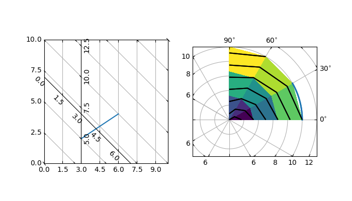
Demonstração de grade curvilínea

Grade personalizada e ticklines.

Este exemplo demonstra como usar GridHelperCurveLinearpara definir grades e linhas de marcação personalizadas aplicando uma transformação na grade. Isso pode ser usado, conforme mostrado no segundo gráfico, para criar projeções polares em uma caixa retangular.

import numpy as np

import matplotlib.pyplot as plt
from matplotlib.projections import PolarAxes
from matplotlib.transforms import Affine2D

from mpl_toolkits.axisartist import angle_helper, Axes, HostAxes
from mpl_toolkits.axisartist.grid_helper_curvelinear import (
    GridHelperCurveLinear)


def curvelinear_test1(fig):
    """
    Grid for custom transform.
    """

    def tr(x, y): return x, y - x
    def inv_tr(x, y): return x, y + x

    grid_helper = GridHelperCurveLinear((tr, inv_tr))

    ax1 = fig.add_subplot(1, 2, 1, axes_class=Axes, grid_helper=grid_helper)
    # ax1 will have ticks and gridlines defined by the given transform (+
    # transData of the Axes).  Note that the transform of the Axes itself
    # (i.e., transData) is not affected by the given transform.
    xx, yy = tr(np.array([3, 6]), np.array([5, 10]))
    ax1.plot(xx, yy)

    ax1.set_aspect(1)
    ax1.set_xlim(0, 10)
    ax1.set_ylim(0, 10)

    ax1.axis["t"] = ax1.new_floating_axis(0, 3)
    ax1.axis["t2"] = ax1.new_floating_axis(1, 7)
    ax1.grid(True, zorder=0)


def curvelinear_test2(fig):
    """
    Polar projection, but in a rectangular box.
    """

    # PolarAxes.PolarTransform takes radian. However, we want our coordinate
    # system in degree
    tr = Affine2D().scale(np.pi/180, 1) + PolarAxes.PolarTransform()
    # Polar projection, which involves cycle, and also has limits in
    # its coordinates, needs a special method to find the extremes
    # (min, max of the coordinate within the view).
    extreme_finder = angle_helper.ExtremeFinderCycle(
        nx=20, ny=20,  # Number of sampling points in each direction.
        lon_cycle=360, lat_cycle=None,
        lon_minmax=None, lat_minmax=(0, np.inf),
    )
    # Find grid values appropriate for the coordinate (degree, minute, second).
    grid_locator1 = angle_helper.LocatorDMS(12)
    # Use an appropriate formatter.  Note that the acceptable Locator and
    # Formatter classes are a bit different than that of Matplotlib, which
    # cannot directly be used here (this may be possible in the future).
    tick_formatter1 = angle_helper.FormatterDMS()

    grid_helper = GridHelperCurveLinear(
        tr, extreme_finder=extreme_finder,
        grid_locator1=grid_locator1, tick_formatter1=tick_formatter1)
    ax1 = fig.add_subplot(
        1, 2, 2, axes_class=HostAxes, grid_helper=grid_helper)

    # make ticklabels of right and top axis visible.
    ax1.axis["right"].major_ticklabels.set_visible(True)
    ax1.axis["top"].major_ticklabels.set_visible(True)
    # let right axis shows ticklabels for 1st coordinate (angle)
    ax1.axis["right"].get_helper().nth_coord_ticks = 0
    # let bottom axis shows ticklabels for 2nd coordinate (radius)
    ax1.axis["bottom"].get_helper().nth_coord_ticks = 1

    ax1.set_aspect(1)
    ax1.set_xlim(-5, 12)
    ax1.set_ylim(-5, 10)

    ax1.grid(True, zorder=0)

    # A parasite axes with given transform
    ax2 = ax1.get_aux_axes(tr)
    # note that ax2.transData == tr + ax1.transData
    # Anything you draw in ax2 will match the ticks and grids of ax1.
    ax1.parasites.append(ax2)
    ax2.plot(np.linspace(0, 30, 51), np.linspace(10, 10, 51), linewidth=2)

    ax2.pcolor(np.linspace(0, 90, 4), np.linspace(0, 10, 4),
               np.arange(9).reshape((3, 3)))
    ax2.contour(np.linspace(0, 90, 4), np.linspace(0, 10, 4),
                np.arange(16).reshape((4, 4)), colors="k")


if __name__ == "__main__":
    fig = plt.figure(figsize=(7, 4))

    curvelinear_test1(fig)
    curvelinear_test2(fig)

    plt.show()