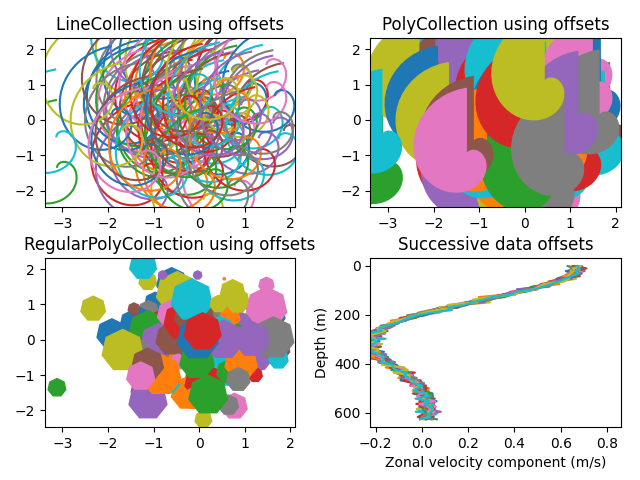
Coleção Line, Poly e RegularPoly com escalonamento automático #

Para as duas primeiras subparcelas, usaremos espirais. Seu tamanho será definido em unidades de plotagem, não em unidades de dados. Suas posições serão definidas em unidades de dados usando os argumentos de palavra-chave offsets e offset_transformLineCollection do e PolyCollection.

A terceira subparcela fará polígonos regulares, com o mesmo tipo de escala e posicionamento das duas primeiras.

A última subtrama ilustra o uso de "offsets=(xo, yo)", ou seja, uma única tupla em vez de uma lista de tuplas, para gerar sucessivamente curvas de deslocamento, com o deslocamento dado em unidades de dados. Esse comportamento está disponível apenas para o LineCollection.

import matplotlib.pyplot as plt
from matplotlib import collections, colors, transforms
import numpy as np

nverts = 50
npts = 100

# Make some spirals
r = np.arange(nverts)
theta = np.linspace(0, 2*np.pi, nverts)
xx = r * np.sin(theta)
yy = r * np.cos(theta)
spiral = np.column_stack([xx, yy])

# Fixing random state for reproducibility
rs = np.random.RandomState(19680801)

# Make some offsets
xyo = rs.randn(npts, 2)

# Make a list of colors cycling through the default series.
colors = [colors.to_rgba(c)
          for c in plt.rcParams['axes.prop_cycle'].by_key()['color']]

fig, ((ax1, ax2), (ax3, ax4)) = plt.subplots(2, 2)
fig.subplots_adjust(top=0.92, left=0.07, right=0.97,
                    hspace=0.3, wspace=0.3)


col = collections.LineCollection(
    [spiral], offsets=xyo, offset_transform=ax1.transData)
trans = fig.dpi_scale_trans + transforms.Affine2D().scale(1.0/72.0)
col.set_transform(trans)  # the points to pixels transform
# Note: the first argument to the collection initializer
# must be a list of sequences of (x, y) tuples; we have only
# one sequence, but we still have to put it in a list.
ax1.add_collection(col, autolim=True)
# autolim=True enables autoscaling.  For collections with
# offsets like this, it is neither efficient nor accurate,
# but it is good enough to generate a plot that you can use
# as a starting point.  If you know beforehand the range of
# x and y that you want to show, it is better to set them
# explicitly, leave out the *autolim* keyword argument (or set it to False),
# and omit the 'ax1.autoscale_view()' call below.

# Make a transform for the line segments such that their size is
# given in points:
col.set_color(colors)

ax1.autoscale_view()  # See comment above, after ax1.add_collection.
ax1.set_title('LineCollection using offsets')


# The same data as above, but fill the curves.
col = collections.PolyCollection(
    [spiral], offsets=xyo, offset_transform=ax2.transData)
trans = transforms.Affine2D().scale(fig.dpi/72.0)
col.set_transform(trans)  # the points to pixels transform
ax2.add_collection(col, autolim=True)
col.set_color(colors)


ax2.autoscale_view()
ax2.set_title('PolyCollection using offsets')

# 7-sided regular polygons

col = collections.RegularPolyCollection(
    7, sizes=np.abs(xx) * 10.0, offsets=xyo, offset_transform=ax3.transData)
trans = transforms.Affine2D().scale(fig.dpi / 72.0)
col.set_transform(trans)  # the points to pixels transform
ax3.add_collection(col, autolim=True)
col.set_color(colors)
ax3.autoscale_view()
ax3.set_title('RegularPolyCollection using offsets')


# Simulate a series of ocean current profiles, successively
# offset by 0.1 m/s so that they form what is sometimes called
# a "waterfall" plot or a "stagger" plot.

nverts = 60
ncurves = 20
offs = (0.1, 0.0)

yy = np.linspace(0, 2*np.pi, nverts)
ym = np.max(yy)
xx = (0.2 + (ym - yy) / ym) ** 2 * np.cos(yy - 0.4) * 0.5
segs = []
for i in range(ncurves):
    xxx = xx + 0.02*rs.randn(nverts)
    curve = np.column_stack([xxx, yy * 100])
    segs.append(curve)

col = collections.LineCollection(segs, offsets=offs)
ax4.add_collection(col, autolim=True)
col.set_color(colors)
ax4.autoscale_view()
ax4.set_title('Successive data offsets')
ax4.set_xlabel('Zonal velocity component (m/s)')
ax4.set_ylabel('Depth (m)')
# Reverse the y-axis so depth increases downward
ax4.set_ylim(ax4.get_ylim()[::-1])


plt.show()

LineCollection usando deslocamentos, PolyCollection usando deslocamentos, RegularPolyCollection usando deslocamentos, deslocamentos de dados sucessivos

Referências

O uso das seguintes funções, métodos, classes e módulos é mostrado neste exemplo:

Galeria gerada por Sphinx-Gallery