Demonstração de contorno #

Ilustre plotagem de contorno simples, contornos em uma imagem com uma barra de cores para os contornos e contornos rotulados.

Veja também o exemplo de imagem de contorno .

import numpy as np
import matplotlib.cm as cm
import matplotlib.pyplot as plt


delta = 0.025
x = np.arange(-3.0, 3.0, delta)
y = np.arange(-2.0, 2.0, delta)
X, Y = np.meshgrid(x, y)
Z1 = np.exp(-X**2 - Y**2)
Z2 = np.exp(-(X - 1)**2 - (Y - 1)**2)
Z = (Z1 - Z2) * 2

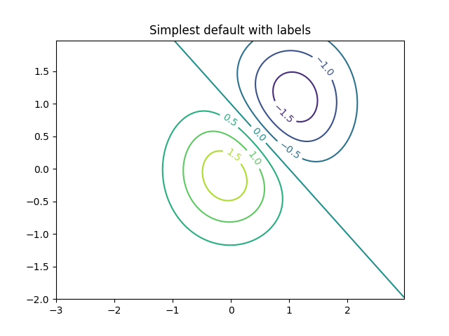
Crie uma plotagem de contorno simples com rótulos usando cores padrão. O argumento embutido para clabel controlará se os rótulos são desenhados sobre os segmentos de linha do contorno, removendo as linhas abaixo do rótulo.

fig, ax = plt.subplots()
CS = ax.contour(X, Y, Z)
ax.clabel(CS, inline=True, fontsize=10)
ax.set_title('Simplest default with labels')

Text(0.5, 1.0, 'Simplest default with labels')

Os rótulos de contorno podem ser colocados manualmente, fornecendo uma lista de posições (na coordenada de dados). Consulte Funções interativas para posicionamento interativo.

fig, ax = plt.subplots()
CS = ax.contour(X, Y, Z)
manual_locations = [
    (-1, -1.4), (-0.62, -0.7), (-2, 0.5), (1.7, 1.2), (2.0, 1.4), (2.4, 1.7)]
ax.clabel(CS, inline=True, fontsize=10, manual=manual_locations)
ax.set_title('labels at selected locations')

Text(0.5, 1.0, 'labels at selected locations')

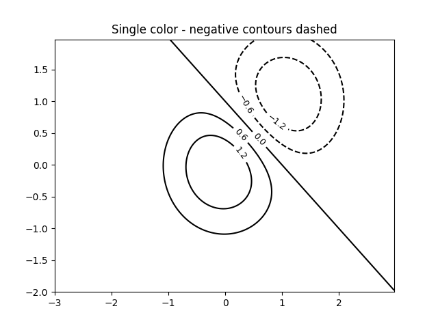
Você pode forçar todos os contornos a serem da mesma cor.

fig, ax = plt.subplots()
CS = ax.contour(X, Y, Z, 6, colors='k')  # Negative contours default to dashed.
ax.clabel(CS, fontsize=9, inline=True)
ax.set_title('Single color - negative contours dashed')

Cor única - contornos negativos tracejados

Text(0.5, 1.0, 'Single color - negative contours dashed')

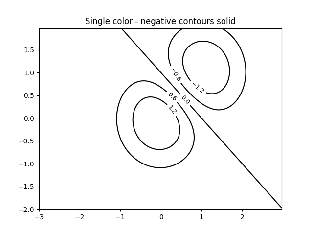
Você pode definir contornos negativos como sólidos em vez de tracejados:

plt.rcParams['contour.negative_linestyle'] = 'solid'
fig, ax = plt.subplots()
CS = ax.contour(X, Y, Z, 6, colors='k')  # Negative contours default to dashed.
ax.clabel(CS, fontsize=9, inline=True)
ax.set_title('Single color - negative contours solid')

Text(0.5, 1.0, 'Single color - negative contours solid')

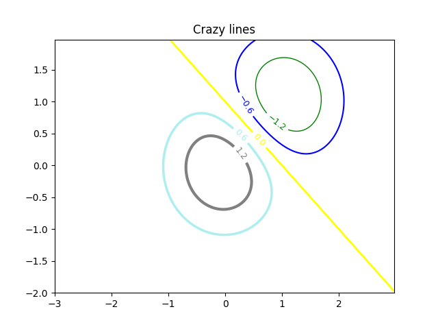
E você pode especificar manualmente as cores do contorno

fig, ax = plt.subplots()
CS = ax.contour(X, Y, Z, 6,
                linewidths=np.arange(.5, 4, .5),
                colors=('r', 'green', 'blue', (1, 1, 0), '#afeeee', '0.5'),
                )
ax.clabel(CS, fontsize=9, inline=True)
ax.set_title('Crazy lines')

Text(0.5, 1.0, 'Crazy lines')

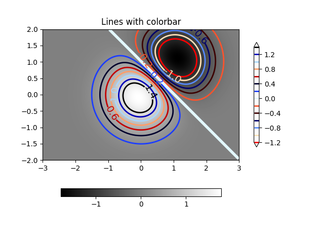
Ou você pode usar um mapa de cores para especificar as cores; o mapa de cores padrão será usado para as linhas de contorno

fig, ax = plt.subplots()
im = ax.imshow(Z, interpolation='bilinear', origin='lower',
               cmap=cm.gray, extent=(-3, 3, -2, 2))
levels = np.arange(-1.2, 1.6, 0.2)
CS = ax.contour(Z, levels, origin='lower', cmap='flag', extend='both',
                linewidths=2, extent=(-3, 3, -2, 2))

# Thicken the zero contour.
CS.collections[6].set_linewidth(4)

ax.clabel(CS, levels[1::2],  # label every second level
          inline=True, fmt='%1.1f', fontsize=14)

# make a colorbar for the contour lines
CB = fig.colorbar(CS, shrink=0.8)

ax.set_title('Lines with colorbar')

# We can still add a colorbar for the image, too.
CBI = fig.colorbar(im, orientation='horizontal', shrink=0.8)

# This makes the original colorbar look a bit out of place,
# so let's improve its position.

l, b, w, h = ax.get_position().bounds
ll, bb, ww, hh = CB.ax.get_position().bounds
CB.ax.set_position([ll, b + 0.1*h, ww, h*0.8])

plt.show()

Referências

O uso das seguintes funções, métodos, classes e módulos é mostrado neste exemplo:

Tempo total de execução do script: ( 0 minutos 2,685 segundos)

Galeria gerada por Sphinx-Gallery