pcolormesh #

axes.Axes.pcolormeshpermite gerar plotagens de estilo de imagem 2D. Note que é mais rápido que o similar pcolor.

import matplotlib.pyplot as plt
from matplotlib.colors import BoundaryNorm
from matplotlib.ticker import MaxNLocator
import numpy as np

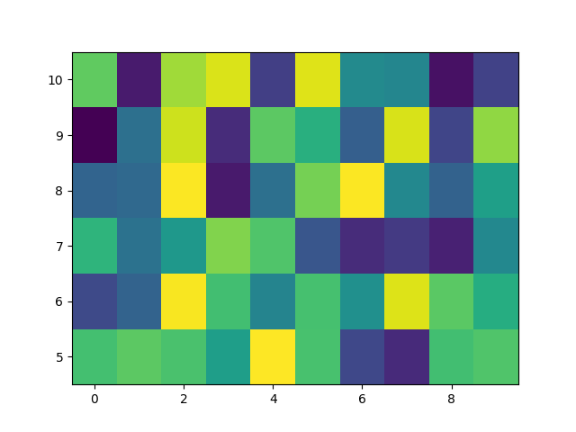
pcolormesh básico #

Geralmente especificamos uma pcolormesh definindo a aresta dos quadriláteros e o valor do quadrilátero. Observe que aqui xey cada um tem um elemento extra do que Z na respectiva dimensão.

np.random.seed(19680801)
Z = np.random.rand(6, 10)
x = np.arange(-0.5, 10, 1)  # len = 11
y = np.arange(4.5, 11, 1)  # len = 7

fig, ax = plt.subplots()
ax.pcolormesh(x, y, Z)

<matplotlib.collections.QuadMesh object at 0x7f2d00aaeef0>

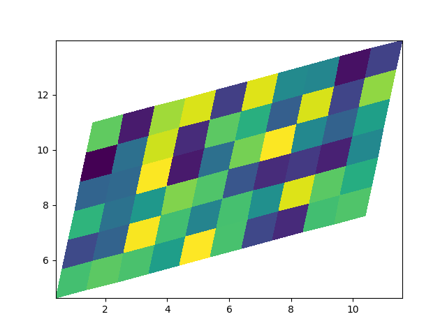
pcolormesh não retilíneo #

Observe que também podemos especificar matrizes para X e Y e ter quadriláteros não retilíneos.

x = np.arange(-0.5, 10, 1)  # len = 11
y = np.arange(4.5, 11, 1)  # len = 7
X, Y = np.meshgrid(x, y)
X = X + 0.2 * Y  # tilt the coordinates.
Y = Y + 0.3 * X

fig, ax = plt.subplots()
ax.pcolormesh(X, Y, Z)

<matplotlib.collections.QuadMesh object at 0x7f2d00c610f0>

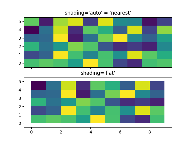
Coordenadas Centradas #

Freqüentemente, um usuário deseja passar X e Y com os mesmos tamanhos de Z para axes.Axes.pcolormesh. Isso também é permitido se shading='auto'for aprovado (padrão definido por rcParams["pcolor.shading"](padrão: 'auto')). Pre Matplotlib 3.3, shading='flat'descartaria a última coluna e linha de Z ; embora isso ainda seja permitido para fins de retrocompatibilidade, um DeprecationWarning é gerado. Se isso é realmente o que você deseja, simplesmente solte a última linha e coluna de Z manualmente:

x = np.arange(10)  # len = 10
y = np.arange(6)  # len = 6
X, Y = np.meshgrid(x, y)

fig, axs = plt.subplots(2, 1, sharex=True, sharey=True)
axs[0].pcolormesh(X, Y, Z, vmin=np.min(Z), vmax=np.max(Z), shading='auto')
axs[0].set_title("shading='auto' = 'nearest'")
axs[1].pcolormesh(X, Y, Z[:-1, :-1], vmin=np.min(Z), vmax=np.max(Z),
                  shading='flat')
axs[1].set_title("shading='flat'")

shading='auto' = 'mais próximo', shading='flat'

Text(0.5, 1.0, "shading='flat'")

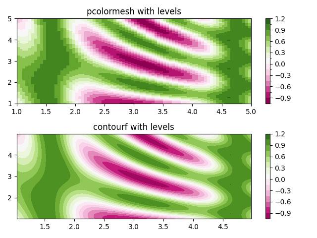
Fazendo níveis usando Normas #

Mostra como combinar instâncias de normalização e mapa de cores para desenhar "níveis" em axes.Axes.pcolor, axes.Axes.pcolormesh e axes.Axes.imshowdigitar plotagens de maneira semelhante ao argumento de palavra-chave de níveis para contorno/contorno.

# make these smaller to increase the resolution
dx, dy = 0.05, 0.05

# generate 2 2d grids for the x & y bounds
y, x = np.mgrid[slice(1, 5 + dy, dy),
                slice(1, 5 + dx, dx)]

z = np.sin(x)**10 + np.cos(10 + y*x) * np.cos(x)

# x and y are bounds, so z should be the value *inside* those bounds.
# Therefore, remove the last value from the z array.
z = z[:-1, :-1]
levels = MaxNLocator(nbins=15).tick_values(z.min(), z.max())


# pick the desired colormap, sensible levels, and define a normalization
# instance which takes data values and translates those into levels.
cmap = plt.colormaps['PiYG']
norm = BoundaryNorm(levels, ncolors=cmap.N, clip=True)

fig, (ax0, ax1) = plt.subplots(nrows=2)

im = ax0.pcolormesh(x, y, z, cmap=cmap, norm=norm)
fig.colorbar(im, ax=ax0)
ax0.set_title('pcolormesh with levels')


# contours are *point* based plots, so convert our bound into point
# centers
cf = ax1.contourf(x[:-1, :-1] + dx/2.,
                  y[:-1, :-1] + dy/2., z, levels=levels,
                  cmap=cmap)
fig.colorbar(cf, ax=ax1)
ax1.set_title('contourf with levels')

# adjust spacing between subplots so `ax1` title and `ax0` tick labels
# don't overlap
fig.tight_layout()

plt.show()

pcolormesh com níveis, contornof com níveis

Referências

O uso das seguintes funções, métodos, classes e módulos é mostrado neste exemplo:

Tempo total de execução do script: ( 0 minutos 1,467 segundos)

Galeria gerada por Sphinx-Gallery