Observação
Clique aqui para baixar o código de exemplo completo
Demonstração Tricontour #
Gráficos de contorno de grades triangulares não estruturadas.
import matplotlib.pyplot as plt
import matplotlib.tri as tri
import numpy as np
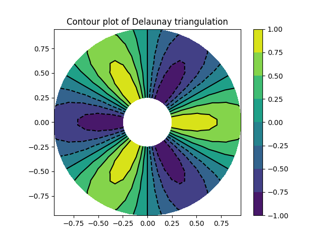
Criar uma triangulação sem especificar os triângulos resulta na triangulação Delaunay dos pontos.
# First create the x and y coordinates of the points.
n_angles = 48
n_radii = 8
min_radius = 0.25
radii = np.linspace(min_radius, 0.95, n_radii)

angles = np.linspace(0, 2 * np.pi, n_angles, endpoint=False)
angles = np.repeat(angles[..., np.newaxis], n_radii, axis=1)
angles[:, 1::2] += np.pi / n_angles

x = (radii * np.cos(angles)).flatten()
y = (radii * np.sin(angles)).flatten()
z = (np.cos(radii) * np.cos(3 * angles)).flatten()

# Create the Triangulation; no triangles so Delaunay triangulation created.
triang = tri.Triangulation(x, y)

# Mask off unwanted triangles.
triang.set_mask(np.hypot(x[triang.triangles].mean(axis=1),
                         y[triang.triangles].mean(axis=1))
                < min_radius)
gráfico pcolor.
fig1, ax1 = plt.subplots()
ax1.set_aspect('equal')
tcf = ax1.tricontourf(triang, z)
fig1.colorbar(tcf)
ax1.tricontour(triang, z, colors='k')
ax1.set_title('Contour plot of Delaunay triangulation')
Text(0.5, 1.0, 'Contour plot of Delaunay triangulation')
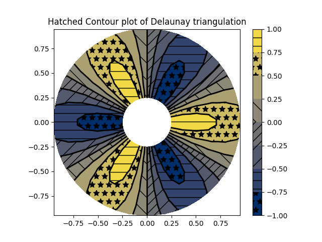
Você também pode especificar padrões de hachura junto com diferentes cmaps.
fig2, ax2 = plt.subplots()
ax2.set_aspect("equal")
tcf = ax2.tricontourf(
    triang,
    z,
    hatches=["*", "-", "/", "//", "\\", None],
    cmap="cividis"
)
fig2.colorbar(tcf)
ax2.tricontour(triang, z, linestyles="solid", colors="k", linewidths=2.0)
ax2.set_title("Hatched Contour plot of Delaunay triangulation")
Text(0.5, 1.0, 'Hatched Contour plot of Delaunay triangulation')
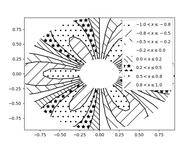
Você também pode gerar padrões de hachura rotulados sem cor.
fig3, ax3 = plt.subplots()
n_levels = 7
tcf = ax3.tricontourf(
    triang,
    z,
    n_levels,
    colors="none",
    hatches=[".", "/", "\\", None, "\\\\", "*"],
)
ax3.tricontour(triang, z, n_levels, colors="black", linestyles="-")


# create a legend for the contour set
artists, labels = tcf.legend_elements(str_format="{:2.1f}".format)
ax3.legend(artists, labels, handleheight=2, framealpha=1)
<matplotlib.legend.Legend object at 0x7f2cfaeb8c10>
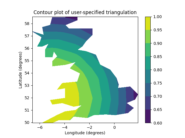
Você pode especificar sua própria triangulação em vez de realizar uma triangulação Delaunay dos pontos, onde cada triângulo é dado pelos índices dos três pontos que compõem o triângulo, ordenados no sentido horário ou anti-horário.
xy = np.asarray([
    [-0.101, 0.872], [-0.080, 0.883], [-0.069, 0.888], [-0.054, 0.890],
    [-0.045, 0.897], [-0.057, 0.895], [-0.073, 0.900], [-0.087, 0.898],
    [-0.090, 0.904], [-0.069, 0.907], [-0.069, 0.921], [-0.080, 0.919],
    [-0.073, 0.928], [-0.052, 0.930], [-0.048, 0.942], [-0.062, 0.949],
    [-0.054, 0.958], [-0.069, 0.954], [-0.087, 0.952], [-0.087, 0.959],
    [-0.080, 0.966], [-0.085, 0.973], [-0.087, 0.965], [-0.097, 0.965],
    [-0.097, 0.975], [-0.092, 0.984], [-0.101, 0.980], [-0.108, 0.980],
    [-0.104, 0.987], [-0.102, 0.993], [-0.115, 1.001], [-0.099, 0.996],
    [-0.101, 1.007], [-0.090, 1.010], [-0.087, 1.021], [-0.069, 1.021],
    [-0.052, 1.022], [-0.052, 1.017], [-0.069, 1.010], [-0.064, 1.005],
    [-0.048, 1.005], [-0.031, 1.005], [-0.031, 0.996], [-0.040, 0.987],
    [-0.045, 0.980], [-0.052, 0.975], [-0.040, 0.973], [-0.026, 0.968],
    [-0.020, 0.954], [-0.006, 0.947], [ 0.003, 0.935], [ 0.006, 0.926],
    [ 0.005, 0.921], [ 0.022, 0.923], [ 0.033, 0.912], [ 0.029, 0.905],
    [ 0.017, 0.900], [ 0.012, 0.895], [ 0.027, 0.893], [ 0.019, 0.886],
    [ 0.001, 0.883], [-0.012, 0.884], [-0.029, 0.883], [-0.038, 0.879],
    [-0.057, 0.881], [-0.062, 0.876], [-0.078, 0.876], [-0.087, 0.872],
    [-0.030, 0.907], [-0.007, 0.905], [-0.057, 0.916], [-0.025, 0.933],
    [-0.077, 0.990], [-0.059, 0.993]])
x = np.degrees(xy[:, 0])
y = np.degrees(xy[:, 1])
x0 = -5
y0 = 52
z = np.exp(-0.01 * ((x - x0) ** 2 + (y - y0) ** 2))

triangles = np.asarray([
    [67, 66,  1], [65,  2, 66], [ 1, 66,  2], [64,  2, 65], [63,  3, 64],
    [60, 59, 57], [ 2, 64,  3], [ 3, 63,  4], [ 0, 67,  1], [62,  4, 63],
    [57, 59, 56], [59, 58, 56], [61, 60, 69], [57, 69, 60], [ 4, 62, 68],
    [ 6,  5,  9], [61, 68, 62], [69, 68, 61], [ 9,  5, 70], [ 6,  8,  7],
    [ 4, 70,  5], [ 8,  6,  9], [56, 69, 57], [69, 56, 52], [70, 10,  9],
    [54, 53, 55], [56, 55, 53], [68, 70,  4], [52, 56, 53], [11, 10, 12],
    [69, 71, 68], [68, 13, 70], [10, 70, 13], [51, 50, 52], [13, 68, 71],
    [52, 71, 69], [12, 10, 13], [71, 52, 50], [71, 14, 13], [50, 49, 71],
    [49, 48, 71], [14, 16, 15], [14, 71, 48], [17, 19, 18], [17, 20, 19],
    [48, 16, 14], [48, 47, 16], [47, 46, 16], [16, 46, 45], [23, 22, 24],
    [21, 24, 22], [17, 16, 45], [20, 17, 45], [21, 25, 24], [27, 26, 28],
    [20, 72, 21], [25, 21, 72], [45, 72, 20], [25, 28, 26], [44, 73, 45],
    [72, 45, 73], [28, 25, 29], [29, 25, 31], [43, 73, 44], [73, 43, 40],
    [72, 73, 39], [72, 31, 25], [42, 40, 43], [31, 30, 29], [39, 73, 40],
    [42, 41, 40], [72, 33, 31], [32, 31, 33], [39, 38, 72], [33, 72, 38],
    [33, 38, 34], [37, 35, 38], [34, 38, 35], [35, 37, 36]])
Em vez de criar um objeto de triangulação, você pode simplesmente passar os arrays x, y e triângulos diretamente para o tripcolor. Seria melhor usar um objeto Triangulação se a mesma triangulação fosse usada mais de uma vez para salvar cálculos duplicados.
fig4, ax4 = plt.subplots()
ax4.set_aspect('equal')
tcf = ax4.tricontourf(x, y, triangles, z)
fig4.colorbar(tcf)
ax4.set_title('Contour plot of user-specified triangulation')
ax4.set_xlabel('Longitude (degrees)')
ax4.set_ylabel('Latitude (degrees)')

plt.show()
Referências
O uso das seguintes funções, métodos, classes e módulos é mostrado neste exemplo:
Tempo total de execução do script: ( 0 minutos 2.280 segundos)